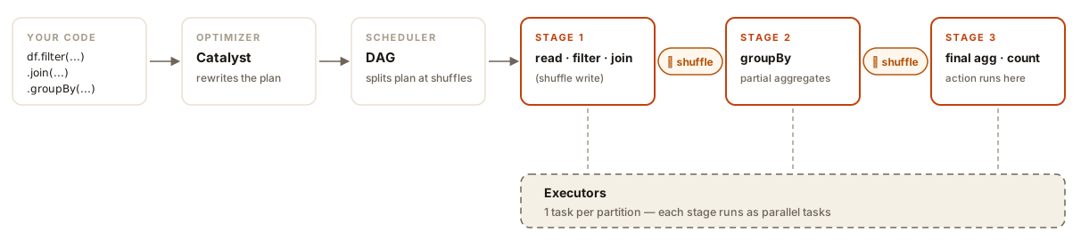
How Spark Really Runs Your DataFrame

Read this pipeline and tell me when Spark does any work:

result = (orders
    .filter(col("amount") > 100)
    .join(customers, "customer_id")
    .groupBy("region").agg(sum("amount").alias("total")))

result.show()

If you said “on the last line” — correct. Everything above it is just Spark taking notes. This laziness is the single most misunderstood thing about Spark, and once you internalize it, caching, checkpointing, and half the performance best practices stop being rules to memorize and start being obvious.

The setup: a tiny dataset

Let’s make it concrete with data small enough to hold in your head:

orders = spark.createDataFrame([
    (1, 101, 250.0), (2, 102, 80.0), (3, 101, 120.0),
    (4, 103, 400.0), (5, 102, 60.0), (6, 101, 90.0),
], ["order_id", "customer_id", "amount"])

customers = spark.createDataFrame([
    (101, "Acme", "East"), (102, "Globex", "West"), (103, "Initech", "East"),
], ["customer_id", "name", "region"])

Six orders, three customers. The pipeline: keep orders over $100, join customer info, total by region. Trivial — which is exactly why it’s a good teaching example. Nothing about the order of execution changes when the data gets big; only the cost of getting it wrong does.

Execution order is not code order

Spark splits every transformation into two kinds:

Narrow — each output partition needs data from exactly one input partition (filter, select, map). These fuse together and stream through memory. Cheap.
Wide — output partitions need data from many input partitions (join, groupBy, distinct, repartition). Spark must shuffle: every machine sends data to every other machine over the network. This is the most expensive thing Spark does, and each shuffle is a stage boundary.

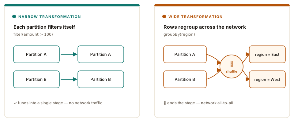
Narrow transformations keep data within each partition; wide transformations shuffle data across partitions — Narrow vs wide: filters stay local, groupBys and joins cross the network.

Walk through it yourself — toggle the broadcast and watch what happens to the stages:

Interactive demo · how Spark orders execution

Broadcast the small customers table — watch the shuffle disappear

1orders = spark.read.table("orders")

Read — nothing runs yet

This only builds a logical plan. No data moves, no tasks launch. Spark is lazy: transformations are just notes about what to do later.

3 stages total — each shuffle is a stage boundary.

Two things to notice. First, the action (.count(), .show(), .write…) is what launches everything; until then, zero bytes have moved. Second, Catalyst (Spark’s optimizer) rewrites your plan before running it — it pushes the filter down to the read and drops columns you never use, so the physical execution order can differ from even the logical one. When in doubt, result.explain() shows you the truth (trimmed here for sanity):

== Physical Plan ==
*(3) HashAggregate(keys=[region], functions=[sum(amount)])
+- Exchange hashpartitioning(region)        ← shuffle: stage boundary
   *(2) HashAggregate(keys=[region], functions=[partial_sum(amount)])
   +- *(2) Project [region, amount]
      +- *(2) BroadcastHashJoin [customer_id]   ← no shuffle: broadcast
         :- *(2) Filter (amount > 100)           ← pushed down, fused
         :  +- *(1) Scan ExistingRDD
         +- BroadcastExchange                   ← small table shipped whole
            +- *(1) Scan ExistingRDD

Read bottom-up: scan, filter fused into the scan, small table broadcast to every executor, partial aggregation per partition, one shuffle for the final grouping. That plan is the whole game.

cache() vs persist(): “remember this answer”

Recompute is Spark’s default. If you use result in two actions, Spark runs the entire pipeline twice — the plan is re-executed from scratch, shuffles and all:

result.count()   # runs the full pipeline
result.show()    # runs the full pipeline AGAIN

cache() says “keep the computed result around”:

result.cache()        # shorthand for persist() with the default level
result.count()        # materializes the cache
result.show()         # reads from memory — no recompute
result.unpersist()    # free it when you're done

persist() is the same idea with a choice of storage level:

Level	Keeps data in	Spills to disk?	Survives executor loss?
`MEMORY_ONLY`	memory, deserialized	no — partitions just get recomputed	no
`MEMORY_AND_DISK` (default)	memory first	yes	no
`DISK_ONLY`	disk	n/a	no
`*_2` variants	as above	as above	yes — 2 replicas

Rule of thumb: use the default unless you have a reason. MEMORY_ONLY on a DataFrame that doesn’t fit means silent recompute of the spilled partitions — the worst of both worlds. And always unpersist() when the cached DataFrame’s job is done; cached data is invisible in the Spark UI’s storage tab only if you go looking, but it absolutely counts against your executors’ memory.

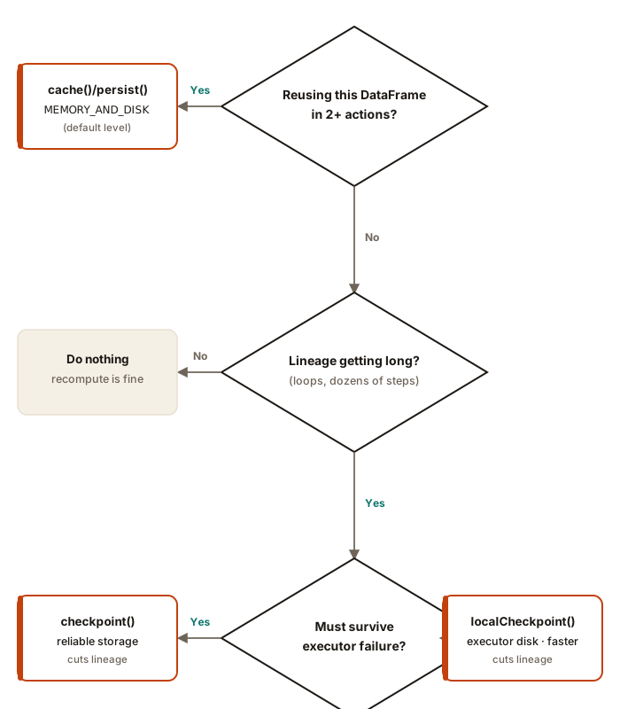
Cache when: the same DataFrame feeds two or more actions, or an iterative algorithm revisits it (ML loops, graph algorithms).

checkpoint(): “cut the lineage”

Every DataFrame remembers its full history — the chain of transformations back to the source. For long iterative pipelines that lineage grows until the driver chokes just planning the job (stack overflows in the DAG are a classic symptom).

checkpoint() truncates the lineage by writing the DataFrame to reliable distributed storage and forgetting how it got there:

spark.sparkContext.setCheckpointDir("dbfs:/checkpoints")

for i in range(50):
    df = df.transform(some_step)

df = df.checkpoint()   # lineage cut here; future plans start fresh
df.count()             # checkpoint materializes on this action

Two properties matter: the write goes to reliable storage (DBFS/S3/HDFS — survives executor failure), and it’s the reliable-but-slow option. There’s also an eager variant, df.checkpoint(eager=True), which materializes immediately instead of waiting for the next action.

localCheckpoint() is the scrappy sibling: it also cuts the lineage, but writes to the executors’ local disks instead of distributed storage. Faster (no network write to S3/HDFS), but if an executor dies, that data is gone and Spark recomputes from the last reliable point. Perfect for iterative ML where a recompute is cheap and you’d rather not pay the distributed-write tax every iteration.

	cache / persist	checkpoint	localCheckpoint
Purpose	avoid recompute	truncate long lineage	truncate long lineage, cheaply
Storage	executor memory/disk	reliable distributed storage	executor local disk
Fault-tolerant	no (except `_2`)	yes	no
Lineage after	kept	cut	cut
Use when	reuse across actions	50+ step iterative pipelines	iterative ML, recompute is cheap

Decision flowchart: reuse across actions leads to cache or persist; long lineage leads to checkpoint or localCheckpoint depending on fault-tolerance needs — Which one do you need? Follow the questions.

Best practices (the ones that actually matter)

These all fall out of the model above — they’re not separate rules:

Filter early, select narrow. Catalyst usually does this for you, but don’t fight it: put filters before joins in your code so the intent is clear, and never select("*") into a shuffle.
Treat shuffles as expensive. Every groupBy, non-broadcast join, and repartition is a network all-to-all. spark.sql.shuffle.partitions defaults to 200 — tune it to your data size, or let Adaptive Query Execution (on by default in Spark 3.x) coalesce them.
Broadcast small tables. Anything under spark.sql.autoBroadcastJoinThreshold (default 10MB) is broadcast automatically; for known-small DataFrames, be explicit: df.join(broadcast(small_df), "key").
Cache reused DataFrames, then unpersist. Two actions on one DataFrame without a cache is the most common accidental 2x slowdown in Spark.
Watch for skew. One giant partition (a null key, a celebrity user-id) makes one task run forever while 199 sit idle. Salt the key or let AQE split it.
Avoid UDFs for row-wise logic. Python UDFs serialize every row out of the JVM; Spark’s native functions stay inside it. Reach for pandas_udf only when vectorization genuinely applies.
Right-size partitions. Aim for ~128MB per partition. Thousands of tiny partitions drown the scheduler in task overhead; a handful of giant ones OOM the executors.
Checkpoint runaway lineages. If your job builds a DataFrame in a loop, checkpoint it — a planning-time stack overflow is a miserable way to learn about lineage.

The takeaway

Spark’s execution model is three sentences: transformations are lazy notes, actions run the plan, shuffles are the unit of cost. Caching answers “don’t recompute this,” checkpointing answers “forget how we got here.” Everything else — broadcast joins, partition tuning, skew handling — is just applied arithmetic on those three sentences. Next time a job is slow, don’t reach for a bigger cluster first. Run explain(), count the exchanges, and ask which shuffle you can kill.